Introduction to dMRI data#
Diffusion imaging probes the random, microscopic movement of water molecules by using MRI sequences that are sensitive to the geometry and environmental organization surrounding these protons. This is a popular technique for studying the white matter of the brain. The diffusion within biological structures, such as the brain, are often restricted due to barriers (e.g., cell membranes), resulting in a preferred direction of diffusion (anisotropy). A typical dMRI scan will acquire multiple volumes (or angular samples), each sensitive to a particular diffusion direction.
Sourced from Dr. A. Rokem, DIPY Workshop 2021
These diffusion directions (or orientations) are a fundamental piece of metadata to interpret dMRI data, as models need to know the exact orientation of each angular sample.
Main elements of a dMRI dataset
A 4D data array, where the last dimension encodes the reconstructed diffusion direction maps.
Tabular data or a 2D array, listing the diffusion directions (
.bvec) and the encoding gradient strength (.bval).
In summary, dMRI involves complex data types that, as programmers, we want to access, query and manipulate with ease.
Python and object oriented programming#
Python is an object oriented programming language. It allows us to represent and encapsulate data types and corresponding behaviors into programming structures called objects.
Data structures
How you feed in data into your algorithm will impose constraints that might completely hinder the implementation of nonfunctional requirements down the line. Therefore, a careful plan must also be thought out for the data structures we are going to handle.
Therefore, let’s leverage Python to create objects that contain dMRI data.
In Python, objects can be specified by defining a class.
In the example code below, we’ve created a class with the name DWI.
To simplify class creation, we’ve also used the magic of a Python library called attrs.
"""Representing data in hard-disk and memory."""
import attr

def _data_repr(value):
    if value is None:
        return "None"
    return f"<{'x'.join(str(v) for v in value.shape)} ({value.dtype})>"


@attr.s(slots=True)
class DWI:
    """Data representation structure for dMRI data."""

    dataobj = attr.ib(default=None, repr=_data_repr)
    """A numpy ndarray object for the data array, without *b=0* volumes."""
    brainmask = attr.ib(default=None, repr=_data_repr)
    """A boolean ndarray object containing a corresponding brainmask."""
    bzero = attr.ib(default=None, repr=_data_repr)
    """A *b=0* reference map, preferably obtained by some smart averaging."""
    gradients = attr.ib(default=None, repr=_data_repr)
    """A 2D numpy array of the gradient table in RAS+B format."""
    em_affines = attr.ib(default=None)
    """
    List of :obj:`nitransforms.linear.Affine` objects that bring
    DWIs (i.e., no b=0) into alignment.
    """

    def __len__(self):
        """Obtain the number of high-*b* orientations."""
        return self.gradients.shape[-1]
This code implements several attributes as well as a behavior - the __len__ method.
The __len__ method is special in Python, as it will be executed when we call the built-in function len() on our object.
Let’s test out the DWI data structure with some simulated data:
# NumPy is a fundamental Python library for working with arrays
import numpy as np

# create a new DWI object, with only gradient information that is random
dmri_dataset = DWI(gradients=np.random.normal(size=(4, 64)))

# call Python's built-in len() function
print(len(dmri_dataset))
64
The output of this print() statement is telling us that this (simulated) dataset has 64 diffusion-weighted samples.
Using the new data representation object#
The code shown above was just a snippet of the DWI class. For simplicity, we will be using the full implementation of this class from our nifreeze package
Under the data/ folder of this book’s distribution, we have stored a sample DWI dataset with filename dwi.h5.
Please note that the file has been minimized by zeroing all but two diffusion-weighted orientation maps.
Let’s get some insights from it:
# import the class from the library
from nifreeze.data.dmri import DWI

# load the sample file
dmri_dataset = DWI.from_filename("../../data/dwi.h5")
print(len(dmri_dataset))
102
In this case, the dataset is reporting to have 102 diffusion-weighted samples.
Python will automatically generate a summary of this object if we just type the name of our new object. This pretty-printing of the object informs us about the data and metadata that, together, compose this particular DWI dataset:
dmri_dataset
DWI(dataobj=<118x118x78x102 (int16)>, affine=<4x4 (float64)>, brainmask=None, motion_affines=None, datahdr=None, bzero=<118x118x78 (int16)>, gradients=<4x10² (float32)>, eddy_xfms=None)
Perhaps, the most interesting aspect of our DWI data structure is that it allows indexed access. That way, we can select data, affine (if initialized), and gradient orientation (b-vector, b-value), for any of the orientations in the data structure:
data, xfm, gradient = dmri_dataset[10]

print(f"shape={data.shape}, gradient={gradient}")
shape=(118, 118, 78), gradient=[-3.1490803e-01 4.7033945e-01 8.2438689e-01 1.0050000e+03]
Visualizing the data#
Exercise
Let’s start by examining the data. We can generate mosaics of DWI data by using the sister tool NiReports:
Hint
We will need to import plot_dwi from NiReports first.
Solution
When calling plot_dwi(), we will be required a 3D data object, and optionally, an affine orientation matrix and a gradient or b-vector.
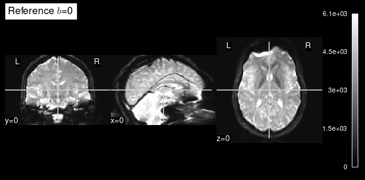
We can access the b=0 reference of the dataset with dmri_dataset.bzero.
This b=0 reference is a map of the signal measured without gradient sensitization, or in other words, when we are not measuring diffusion in any direction.
The b=0 map can be used by diffusion modeling as the reference to quantify the signal drop at every voxel and given a particular orientation gradient.
We can also get some insight into how a particular diffusion-weighted orientation looks like by selecting them with the argument index.
Exercise
Try calling plot_dwi with an index of 10 or 100.
Solution
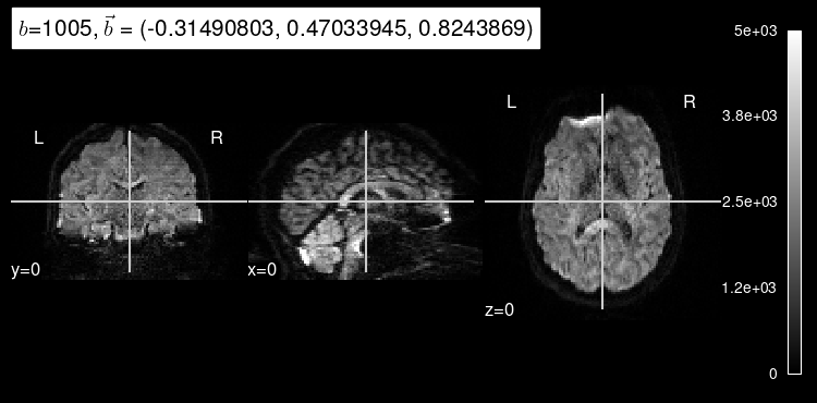
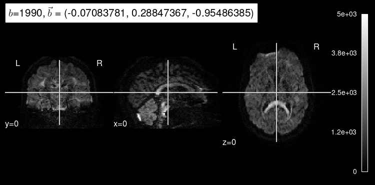
Diffusion that exhibits directionality in the same direction as the gradient results in a loss of signal. As we can see, diffusion-weighted images consistently drop almost all signal in voxels filled with cerebrospinal fluid because there, water diffusion is free (isotropic) regardless of the direction that is being measured.
We can also see that the images at indexes 10 and 100 have different gradient strength (”b-value”). The higher the magnitude of the gradient, the more diffusion that is allowed to occur, indicated by the overall decrease in signal intensity. Stronger gradients yield diffusion maps with substantially lower SNR (signal-to-noise ratio), as well as larger distortions derived from the so-called “Eddy-currents”.
Visualizing the gradient information#
Our DWI object stores the gradient information in the gradients attribute.
Exercise
Let’s see the shape of the gradient information.
Solution
We get a \(4\times102\) – three spatial coordinates (\(b_x\), \(b_y\), \(b_z\)) of the unit-norm “b-vector”, plus the gradient sensitization magnitude (the “b-value”), with a total of 102 different orientations for the case at hand.
Exercise
Try printing the gradient information to see what it contains.
Remember to transpose (.T) the array.
Solution
Later, we’ll refer to this array as the gradient table.
It consists of one row per diffusion-weighted image, with each row consisting of 4 values corresponding to [ R A S+ b ].
[ R A S+ ] are the components of the gradient direction. Note that the directions have been re-oriented with respect to world space coordinates. For more information on this, refer to the Affine section in The extra mile.
The last column, b, reflects the timing and strength of the gradients in units of s/mm².
To get a better sense of which gradient directions were sampled, let’s plot them!
from nireports.reportlets.modality.dwi import plot_gradients

plot_gradients(dmri_dataset.gradients.T);

We’ve projected all of the gradient directions onto the surface of a sphere, with each unique gradient strength colour-coded. Darkest hues correspond to the lowest b-values and brighter to the highest.
Next steps: diffusion modeling#
By modeling the diffusion signal, the acquired images can provide measurements which are related to the microscopic changes and estimate white matter trajectories.