Reducing the dimensionality of the metrics

First, let’s load the ABIDE dataset, and apply the site-wise normalization.

from mriqc_learn.datasets import load_dataset
from mriqc_learn.models.preprocess import SiteRobustScaler

(train_x, train_y), _ = load_dataset(split_strategy="none")
train_x = train_x.drop(columns=[
    "size_x",
    "size_y",
    "size_z",
    "spacing_x",
    "spacing_y",
    "spacing_z",
])
numeric_columns = train_x.columns.tolist()
train_x["site"] = train_y.site

# Harmonize between sites
scaled_x = SiteRobustScaler(unit_variance=True).fit_transform(train_x)

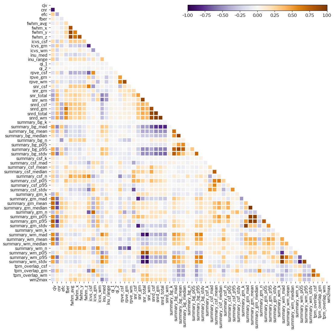
We have a total of 62 features (i.e., metrics), and many of them are related (e.g., region-wise SNR calculations, or different ways of estimating a particular measure). Highly correlated (either positive or negatively correlated) are not adding much information about the image to one another. We therefore expect to see high (negative and positive) correlations between different metrics:

from mriqc_learn.viz import metrics

metrics.plot_corrmat(scaled_x[numeric_columns].corr(), figsize=(12, 12));

Principal Components Analysis (PCA)

PCA is a fundamental statistical decomposition of data that was proposed to resolve the problem of source separation. By using a few of the largest components, the signal can effectively be reduced from our initial 62 channels into a much lower number. We will be using scikit-learn and scipy in this example:

from scipy import stats
from sklearn.decomposition import PCA

First we instantiate the model without limiting the number of components and fit the model to the numeric columns (i.e., without site of origin) of our dataframe:

pca_model = PCA(n_components=None).fit(scaled_x[numeric_columns])

Now let’s investigate this PCA model. To make an educated guess of a sufficient number of components for properly representing the data, we typically look at an elbow plot showing the variance explained vs. the number of components.

fig = plt.figure(figsize=(15,6))
plt.plot(np.cumsum(pca_model.explained_variance_ratio_ * 100), "-x")
plt.ylabel("Cumulative variance explained [%]")
plt.xlabel("Number of components")
xticks = np.arange(0, pca_model.explained_variance_ratio_.size, dtype=int)
plt.xticks(xticks)
plt.gca().set_xticklabels(xticks + 1)
yticks = np.linspace(92.0, 100.0, num=5)
plt.yticks(yticks)
plt.gca().set_yticklabels([f"{v:.2f}" for v in yticks]);

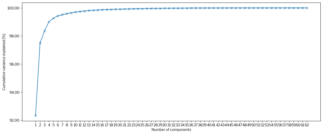
We can see that the first four components account for 99% of the variance, which is pretty high. Let’s then choose to keep four components from now on:

n_components = 4

Components are no more than linear decomposition of the original metrics, so let’s now look at the coefficients that correspond to the IQMs for each of those first four components:

basis = pca_model.components_[:n_components,:]
fig, axs = plt.subplots(1, 4, sharex=False, sharey=False, figsize=(24, 6))
for k in range(basis.shape[0]):
    axs[k].plot(np.abs(basis[k,:]), "x")
    axs[k].set_title(f"Component {k + 1}")

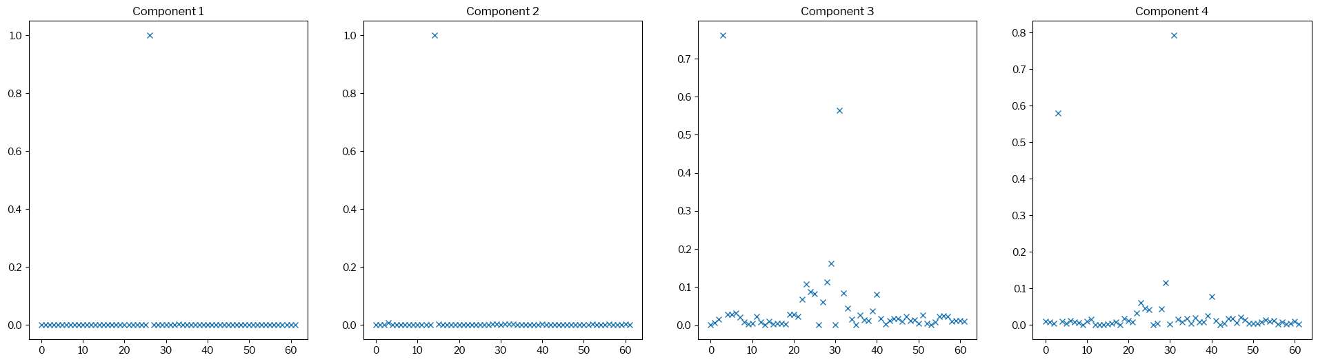
The first two components are basically aligned with one original metric each. The second two are more composite of several metrics, but again only two features weight above 0.5, in both cases.

Let’s refit the model with the limitation of 4 components, and project our original data onto the new four-dimensional space.

iqm_reduced = PCA(n_components=n_components).fit_transform(
  scaled_x[numeric_columns]
)
components = pd.DataFrame(iqm_reduced, columns=[f"PC{i}" for i in range(1, n_components + 1)])
components["site"] = scaled_x["site"].values
components

	PC1	PC2	PC3	PC4	site
0	-6.947685	-1.913501	-2.438583	-1.045978	PITT
1	-4.373293	-1.723562	-3.803143	-0.219094	PITT
2	-7.242282	-0.484759	0.994786	-1.353356	PITT
3	-7.176610	-2.449517	-1.096229	-1.298902	PITT
4	-7.139118	0.812015	3.909931	-0.496021	PITT
...	...	...	...	...	...
1096	-6.680810	-2.407759	1.327108	-0.842666	SBL
1097	-6.512875	-1.902763	-1.429952	-0.977564	SBL
1098	-6.562521	-0.946969	-0.655515	-1.599633	SBL
1099	-6.954292	-1.025446	0.491796	-2.239100	MAX_MUN
1100	-6.546351	-2.045979	0.338038	-1.860973	MAX_MUN

1101 rows × 5 columns

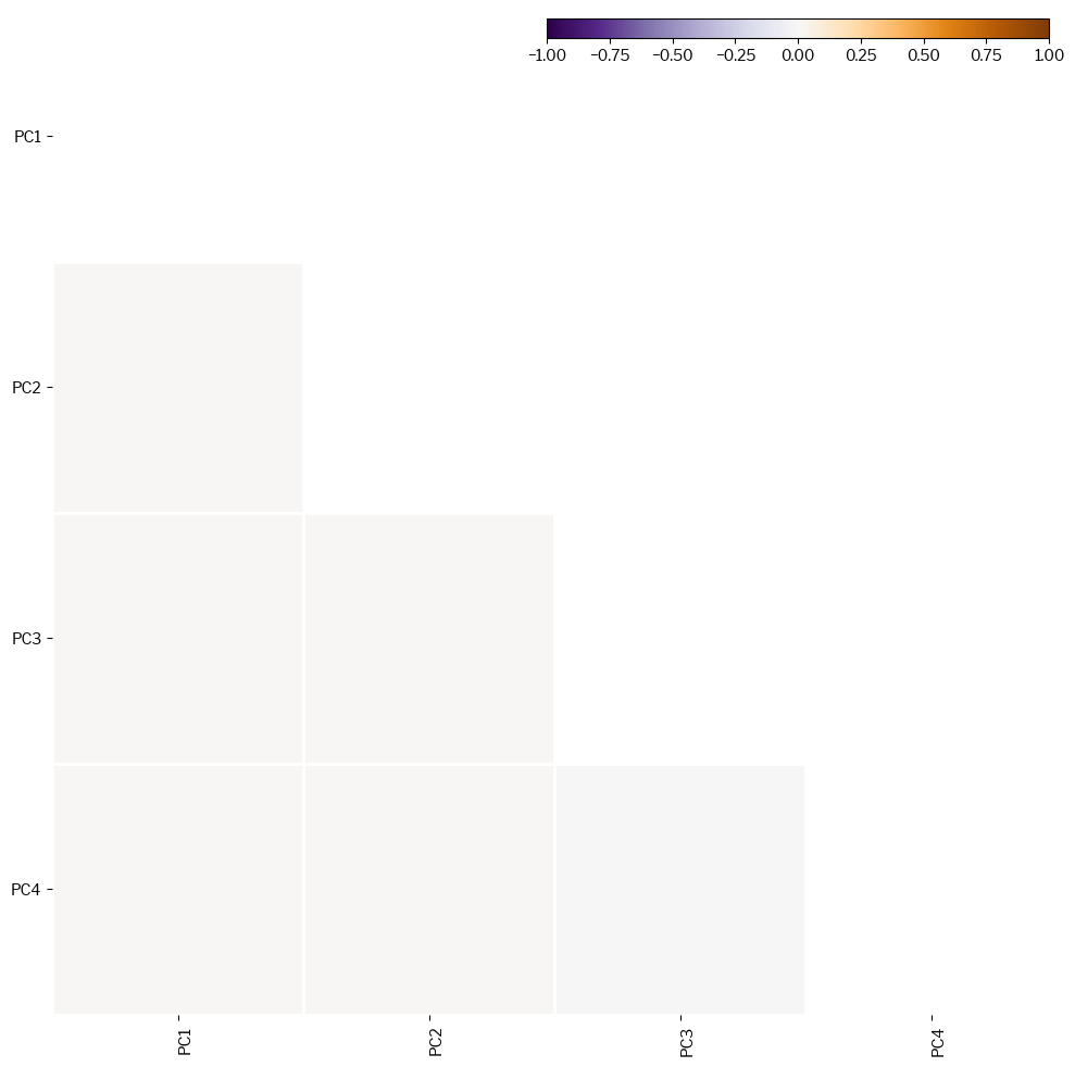
The components should not be correlated:

components.drop(columns=["site"])
metrics.plot_corrmat(components.corr(), figsize=(12, 12));

/tmp/ipykernel_5506/3560390741.py:2: FutureWarning: The default value of numeric_only in DataFrame.corr is deprecated. In a future version, it will default to False. Select only valid columns or specify the value of numeric_only to silence this warning.
  metrics.plot_corrmat(components.corr(), figsize=(12, 12));

Thanks

We thank Céline Provins for the original notebook on which this section is based.