Understanding IQMs generated by MRIQC

The mriqc-learn package comes with some example data for users, derived from the MRIQC paper. First, we will be using a dataset containing IQMs generated on the open-access ABIDE I dataset which contains manual assessments by human raters. Let’s explore the dataset:

# 1. mriqc-learn comes with a convenience data loader, you'll need to first import it.
from mriqc_learn.datasets import load_dataset

# 2. Once imported, let's pull up some data
(train_x, train_y), _ = load_dataset(split_strategy="none")

# 3. Remove non-informative IQMs (image size and spacing)
train_x = train_x.drop(columns=[
    "size_x",
    "size_y",
    "size_z",
    "spacing_x",
    "spacing_y",
    "spacing_z",
])

# 4. Keep a list of numeric columns before adding the site as a column
numeric_columns = train_x.columns.tolist()

With the argument split_strategy="none" we are indicating that we want to obtain the full dataset, without partitioning it in any ways. That means variable train_x will contain features (in other words, the actual IQMs) and train_y contains manual assessments, for 1101 T1-weighted MRI images of ABIDE I. Both data tables train_x and train_y have the structure of Pandas DataFrames.

In order to investigate those “site-effects”, let’s add a column to train_x with site information:

train_x["site"] = train_y.site

These sites correspond to the following acquisition parameters:

A first look on the dataset

Lets now have a first quick look over the data:

train_x

	cjv	cnr	efc	fber	fwhm_avg	fwhm_x	fwhm_y	fwhm_z	icvs_csf	icvs_gm	...	summary_wm_median	summary_wm_n	summary_wm_p05	summary_wm_p95	summary_wm_stdv	tpm_overlap_csf	tpm_overlap_gm	tpm_overlap_wm	wm2max	site
0	0.383747	3.259968	0.609668	181.619858	3.944888	3.959924	4.039157	3.835584	0.199774	0.449138	...	1000.013428	189965.0	908.938904	1079.413428	51.778980	0.225944	0.525072	0.540801	0.540213	PITT
1	0.574080	2.279440	0.606361	172.500031	3.992397	3.877495	4.173095	3.926602	0.203301	0.429628	...	1000.033569	187992.0	901.788293	1120.833569	67.136932	0.223374	0.521399	0.560238	0.571425	PITT
2	0.314944	3.998569	0.577123	273.688171	4.016382	4.066009	4.092888	3.890248	0.201591	0.446495	...	1000.015198	188213.0	913.847803	1067.003662	46.623932	0.233414	0.531020	0.556496	0.612655	PITT
3	0.418505	3.050534	0.571343	237.531143	3.601741	3.629409	3.627568	3.548246	0.190612	0.468255	...	1000.005981	146722.0	872.409717	1083.139264	63.131420	0.227282	0.528115	0.526254	0.600312	PITT
4	0.286560	4.214082	0.550083	427.042389	3.808350	3.839143	3.841085	3.744823	0.162421	0.505201	...	1000.004150	162584.0	900.433481	1069.912750	50.874363	0.195150	0.543591	0.531606	0.603308	PITT
...	...	...	...	...	...	...	...	...	...	...	...	...	...	...	...	...	...	...	...	...	...
1096	0.428731	3.030323	0.789654	2519.999512	3.176760	3.166740	3.359990	3.003550	0.169851	0.424819	...	1000.034668	241117.0	902.529590	1088.244409	56.683868	0.162535	0.476992	0.536843	0.537140	SBL
1097	0.610845	2.155928	0.800116	1769.720093	3.209497	3.164760	3.381280	3.082450	0.170732	0.405536	...	1000.039429	251136.0	903.951080	1093.323273	57.789230	0.193376	0.465232	0.545695	0.564010	SBL
1098	0.461773	2.794299	0.789859	2248.858398	3.149920	3.112220	3.326700	3.010840	0.165501	0.441190	...	1000.036438	209298.0	891.934216	1093.973322	61.108639	0.198508	0.497137	0.523571	0.564865	SBL
1099	0.457718	2.862913	0.706924	114.865364	3.486750	3.421200	3.881950	3.157100	0.209701	0.381839	...	999.990356	234957.0	904.907922	1101.429980	60.045422	0.235618	0.477310	0.563352	0.534626	MAX_MUN
1100	0.419648	3.129415	0.783152	116.484947	3.579490	3.538990	3.991800	3.207680	0.215531	0.402868	...	1000.005981	244797.0	904.572144	1095.835376	58.381458	0.227491	0.492317	0.549036	0.573174	MAX_MUN

1101 rows × 63 columns

This first look is not very informative - there’s no way we can pick any of the structure in our dataset.

First, let’s investigate the number of metrics:

len(numeric_columns)

62

Let’s now make use of one plotting utility of mriqc-learn, and observe the structure:

# 1. Let's import a module containing visualization tools for IQMs
from mriqc_learn.viz import metrics

# 2. Plot the dataset
fig1 = metrics.plot_batches(train_x)

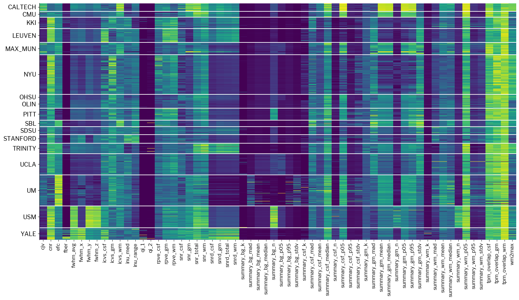
The plot above is clearly blocky, very well aligned with the different acquisition sites that are comprehended.

Homogenizing across sites

One first thought to make these IQMs more homogeneous would be to site-wise standardize them. This means, for each site, calculate mean and standard deviation and apply them to convert IQMs to zero-mean, unit-variance distributions. mriqc-learn has a filter (derived from, and compatible with scikit-learn) to do this:

# Load the filter
from mriqc_learn.models.preprocess import SiteRobustScaler

# Plot data after standardization
standardized_x = SiteRobustScaler(unit_variance=True).fit_transform(train_x)
fig2 = metrics.plot_batches(standardized_x)

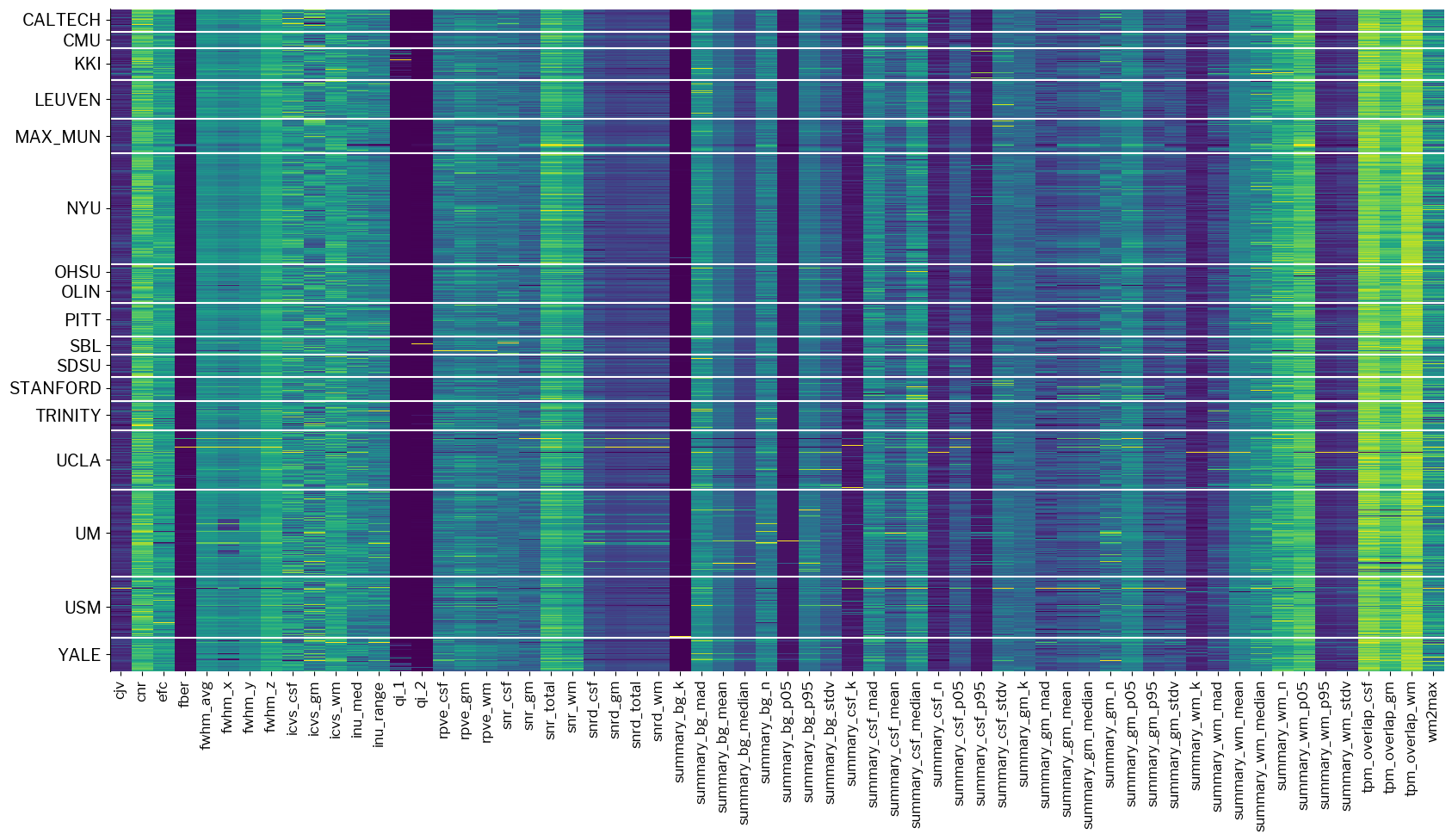
Now the plot is not so blocky.

A different way of looking at this is plotting histograms of some metrics, with the original and the standardized version represented side-by-side. For example, this would be the picture for the coefficient of joint variation (CJV), which is passed in as the metric argument:

metrics.plot_histogram(train_x, standardized_x, metric="cjv");

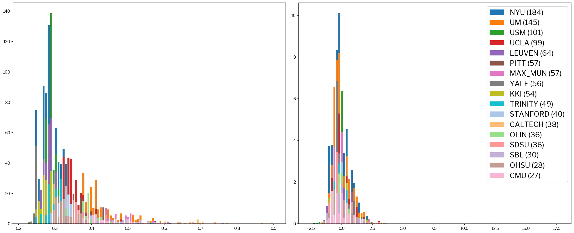
It is clear that, on the left, sites tend to cluster in regions of the spread of values (X-axis). Conversely, on the right-hand histogram, sites overlap much more and form together some sort of gaussian distribution.

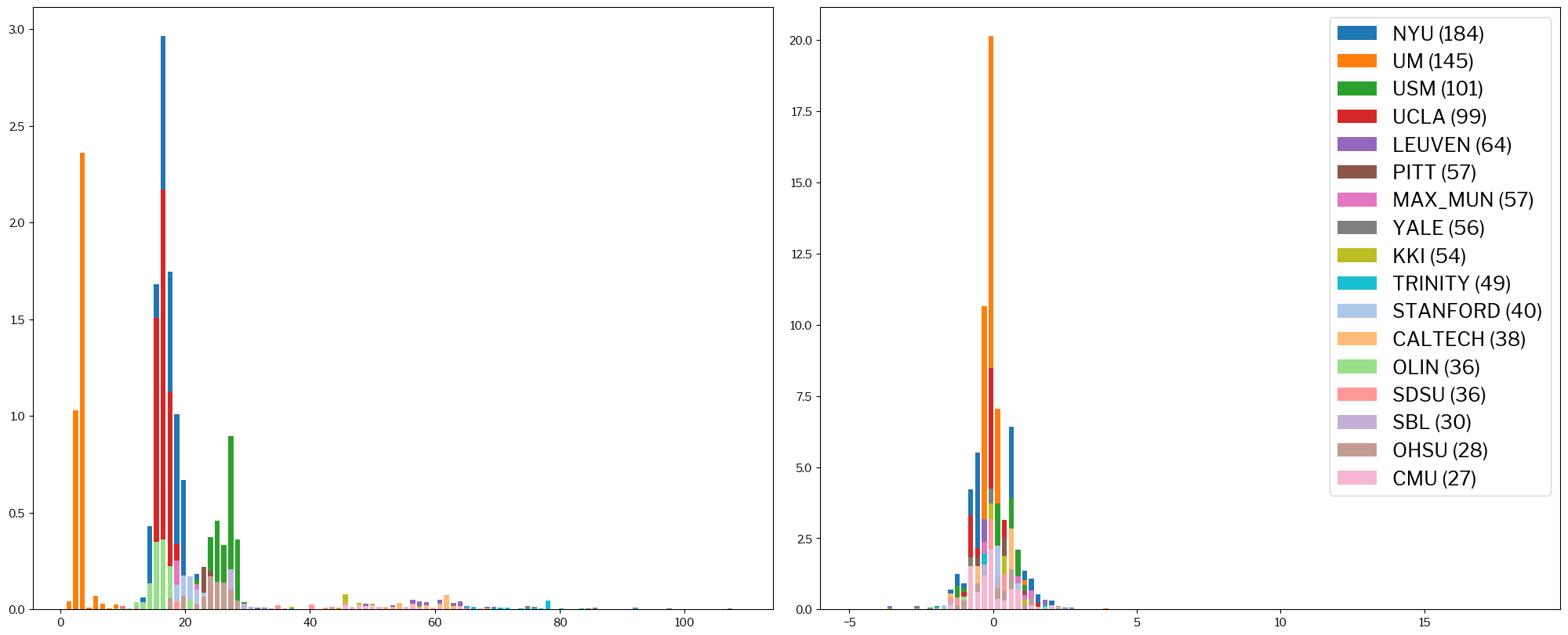
The situation is even more clear for the following definition of SNR (snrd_total):

metrics.plot_histogram(train_x, standardized_x, metric="snrd_total");

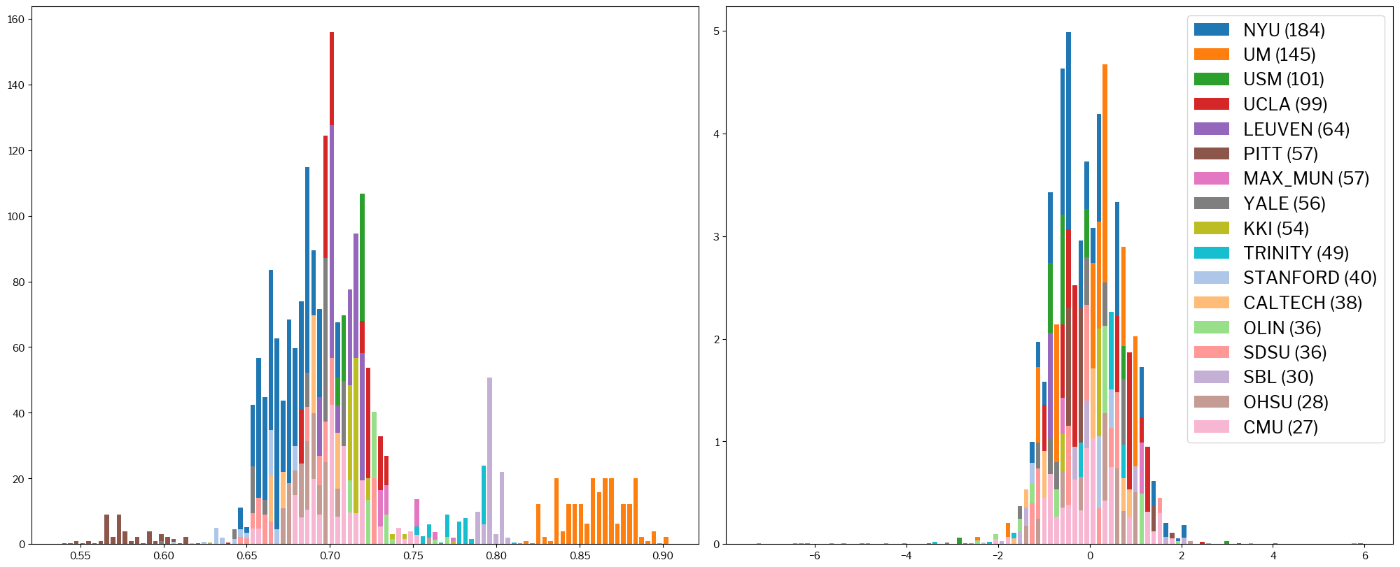
Now, this is how the entropy-focus criterion (EFC) looks like:

metrics.plot_histogram(train_x, standardized_x, metric="efc");

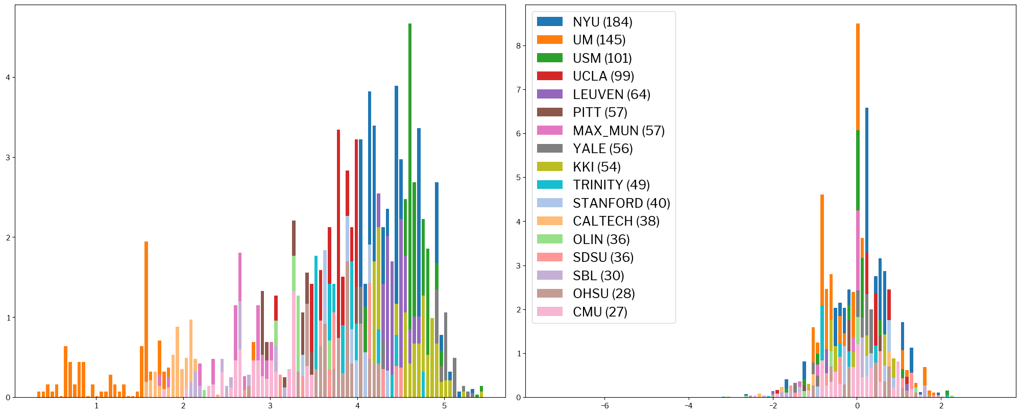
Finally, a look on a very commonly used parameter, the contrast-to-noise ratio (CNR):

metrics.plot_histogram(train_x, standardized_x, metric="cnr");

What’s the problem?

Any model we train on those features heavily reliant on the site of acquisition will rather pick up the site where the image was acquired than the quality (which is our target). This is so because perceived image quality by humans (the target outcome we want to predict) is very correlated with the site of acquisition. In other words, our machine-learning model will operate like a human would do: given that this site produces mostly poor images, I will assume all images coming from it are poor.

At this point, it is clear that we are about to try training models on rather noisy features, which also show strong biases correlated with the acquisition site.

Unfortunately, there are further complications. Indeed, the targets (image quality assessments) that we can use in training are also very noisy.

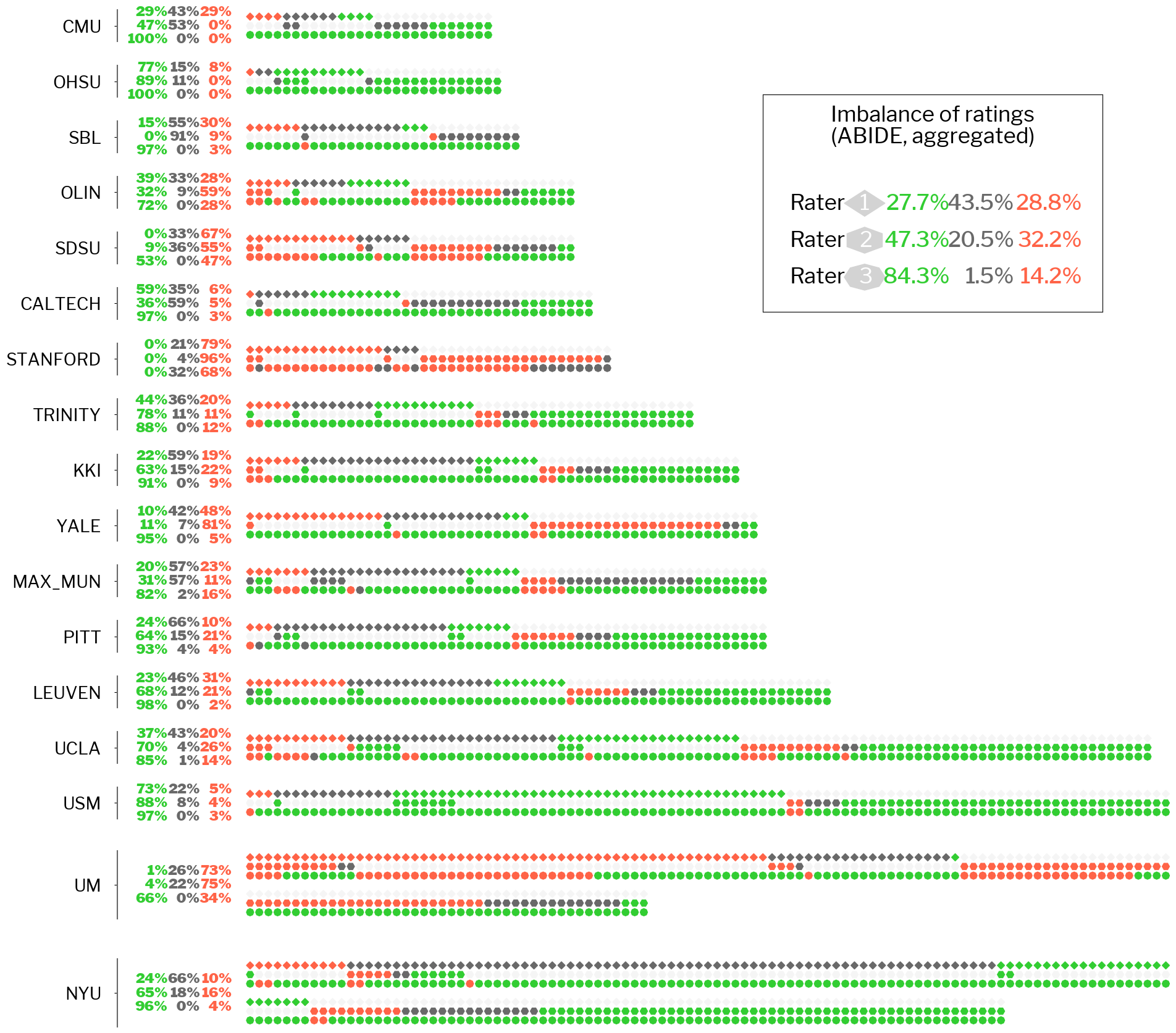
Target labels: manual ratings by humans

Let’s go further in exploring the effect of labels noise, by now focusing our attention on the dataset targets (train_y).

from mriqc_learn.viz import ratings
ratings.raters_variability_plot(train_y);