Methods and implementation
SDCFlows defines a clear API that divides the problem of susceptibility distortions (SD) into two stages:
Estimation: the MRI acquisitions in the protocol for SD are discovered and preprocessed to estimate a map of B0 non-uniformity in Hz (\(\Delta B_0\)). The theory behind these distortions is well described in the literature ([Jezzard1995], [Hutton2002]), and further discussed below (see a summary in Fig. 1). SDCFlows builds on freely-available software to implement three major strategies for estimating \(\Delta B_0\) (Eq. \(\eqref{eq:fieldmap-1}\)). These strategies are described below, and implemented within
sdcflows.workflows.fit.Application: the B-Spline basis coefficients used to represent the estimated \(\Delta B_0\) map mapped into the target EPI scan to be corrected, and a displacement field in NIfTI format that is compatible with ANTs is interpolated from the B-Spline basis. The voxel location error along the PE will be proportional to \(\Delta B_0 \cdot T_\text{ro}\), where \(T_\text{ro}\) is the total readout time of the target EPI (Fig. 1). The implementation of these workflows is found in the submodule
sdcflows.workflows.apply.
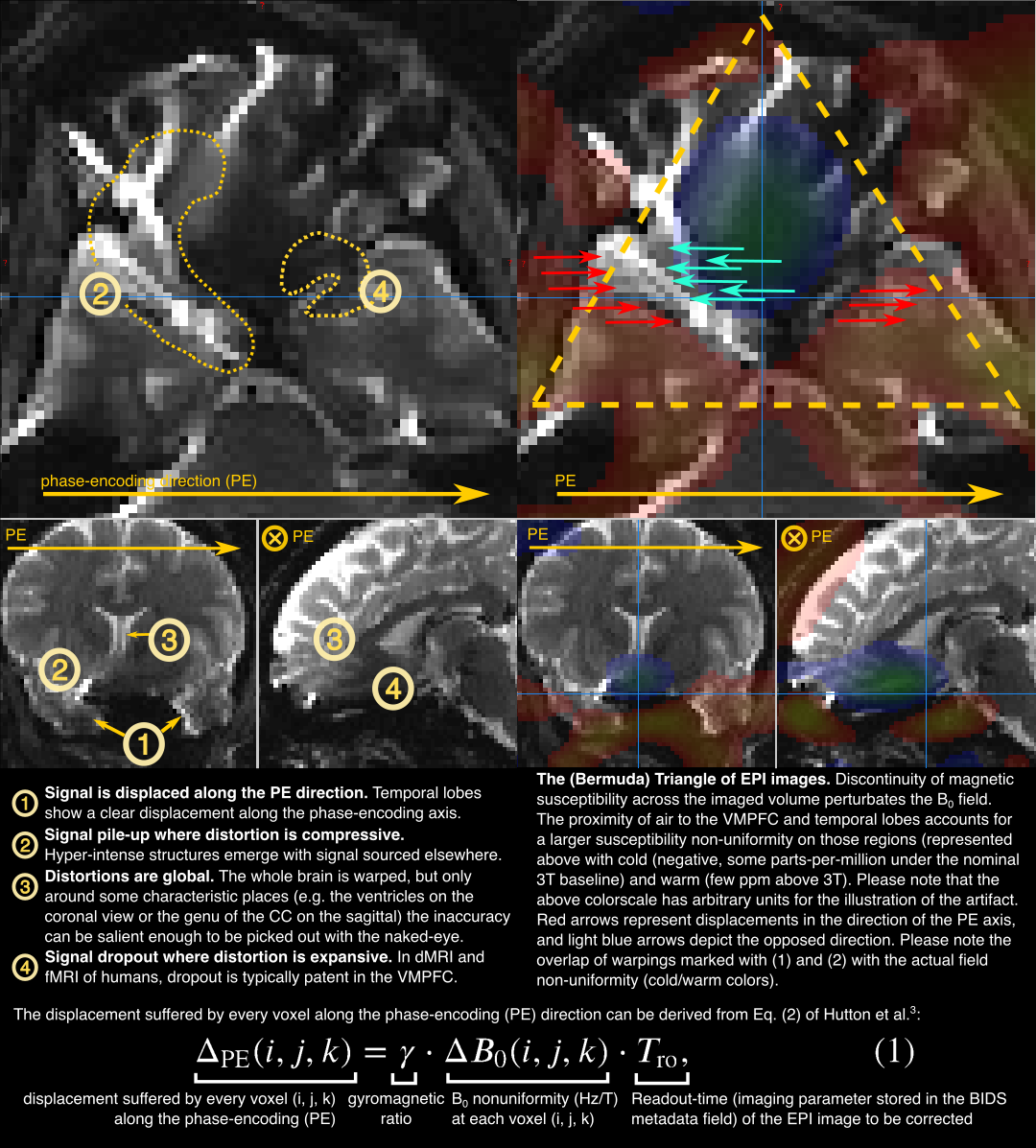
Fig. 1 Susceptibility distortions in a nutshell
BIDS Specification
See the section Echo-planar imaging and *B0* mapping.
Fieldmap estimation: theory and methods
The displacement suffered by every voxel along the PE direction can be derived from Eq. (2) of [Hutton2002]:
where \(\Delta_\text{PE} (i, j, k)\) is the voxel-shift map (VSM) along the PE direction, \(\gamma\) is the gyromagnetic ratio of the H proton in Hz/T (\(\gamma = 42.576 \cdot 10^6 \, \text{Hz} \cdot \text{T}^\text{-1}\)), \(\Delta B_0 (i, j, k)\) is the fieldmap variation in T (Tesla), and \(T_\text{ro}\) is the readout time of one slice of the EPI dataset we want to correct for distortions.
Let \(V\) represent the fieldmap in Hz (or equivalently, voxel-shift-velocity map, as Hz are equivalent to voxels/s), with \(V(i,j,k) = \gamma \cdot \Delta B_0 (i, j, k)\), then, introducing the voxel zoom along the phase-encoding direction, \(s_\text{PE}\), we obtain the nonzero component of the associated displacements field \(\Delta D_\text{PE} (i, j, k)\) that unwarps the target EPI dataset:
Direct B0 mapping sequences
BIDS Specification
See the section Types of fieldmaps - Case 3: Direct field mapping in the BIDS specification.
Some MR schemes such as SEI can directly reconstruct an estimate of the fieldmap in Hz, \(V(i,j,k)\). These fieldmaps are described with more detail here.
Phase-difference B0 estimation
BIDS Specification
See the section Types of fieldmaps - Case 2: Two phase maps and two magnitude images in the BIDS specification.
Some scanners produce one phasediff map, where the drift between the two echos has
already been calculated, see the section
Types of fieldmaps - Case 1: Phase-difference map and at least one magnitude image.
The fieldmap variation in T, \(\Delta B_0 (i, j, k)\), that is necessary to obtain \(\Delta_\text{PE} (i, j, k)\) in Eq. \(\eqref{eq:fieldmap-1}\) can be calculated from two subsequent GRE echoes, via Eq. (1) of [Hutton2002]:
where \(\Delta \Theta (i, j, k)\) is the phase-difference map in radians, and \(\Delta\text{TE}\) is the elapsed time between the two GRE echoes.
For simplicity, the «voxel-shift-velocity map» \(V(i,j,k)\), which we can introduce in Eq. \(\eqref{eq:fieldmap-2}\) to directly obtain the displacements field, can be obtained as:
This calculation is further complicated by the fact that \(\Theta_i\) (and therefore, \(\Delta \Theta\)) are clipped (or wrapped) within the range \([0 \dotsb 2\pi )\). It is necessary to find the integer number of offsets that make a region continuously smooth with its neighbors (phase-unwrapping, [Jenkinson2003]).
PEPOLAR techniques
BIDS Specification
See the section Types of fieldmaps - Case 4: Multiple phase encoded directions (“pepolar”).
Alternatively, it is possible to estimate the field by exploiting the symmetry of the
distortion when the PE polarity is reversed.
SDCFlows integrates two implementations based on FSL topup [Andersson2003],
and AFNI 3dQwarp [Cox1997].
By default, FSL topup will be used.
Fieldmap-less approaches
Many studies acquired (especially with legacy MRI protocols) do not have any information to estimate susceptibility-derived distortions. In the absence of data with the specific purpose of estimating the \(B_0\) inhomogeneity map, researchers resort to nonlinear registration to an «anatomically correct» map of the same individual (normally acquired with T1w, or T2w sequences). One of the most prominent proposals of this approach is found in [Studholme2000].
SDCFlows includes an (experimental) procedure, based on nonlinear image registration with ANTs’ symmetric normalization (SyN) technique. This workflow takes a skull-stripped T1w image and a reference EPI image, and estimates a field of nonlinear displacements that accounts for susceptibility-derived distortions. To more accurately estimate the warping on typically distorted regions, this implementation uses an average \(B_0\) mapping described in [Treiber2016]. The implementation is a variation on those developed in [Huntenburg2014] and [Wang2017].
The process is divided in two steps.
First, the two images to be aligned (anatomical and one or more EPI sources) are prepared for
registration, including a linear pre-alignment of both, calculation of a 3D EPI reference map,
intensity/histogram enhancement, and deobliquing (meaning, for images where the physical
coordinates axes and the data array axes are not aligned, the physical coordinates are
rotated to align with the data array).
Such a preprocessing is implemented in
init_syn_preprocessing_wf().
Second, the outputs of the preprocessing workflow are fed into
init_syn_sdc_wf(),
which executes the nonlinear, SyN registration.
To aid the Mattes mutual information cost function, the registration scheme is set up
in multi-channel mode, and laplacian-filtered derivatives of both anatomical and EPI
reference are introduced as a second registration channel.
The optimization gradients of the registration process are weighted, so that deformations
effectively possible only along the PE axis.
Given that ANTs’ registration framework performs on physical coordinates, it is necessary
that input images are not oblique.
The anatomical image is used as fixed image, and therefore, the registration process
estimates the transformation function from unwarped (anatomically correct) coordinates
to distorted coordinates.
If fed into antsApplyTransforms, the resulting transform will effectively unwarp a distorted
EPI given as input into its unwarped mapping.
The estimated transform is then converted into a \(B_0\) fieldmap in Hz, which can be
stored within the derivatives folder.
Danger
This procedure is experimental, and the outcomes should be scrutinized one-by-one and used with caution. Feedback will be enthusiastically received.
Other (unsupported) approaches
There exist some alternative options to estimate the fieldmap, such as mapping the point-spread-function [Zaitsev2004], or by means of nonlinear registration of brain surfaces onto the distorted EPI data [Esteban2016].
Estimation tooling
The workflows provided by sdcflows.workflows.fit make use of several utilities.
The cornerstone of these tools is the fieldmap representation with B-Splines
(sdcflows.interfaces.bspline).
B-Splines are well-suited to plausibly smooth the fieldmap and provide a compact
representation of the field with fewer parameters.
This representation is also more accurate in the case the images that were used for estimation
are not aligned with the target images to be corrected because the fieldmap is not directly
interpolated in the projection, but rather, the position of the coefficients in space is
updated and then the fieldmap reconstructed.
Unwarping the distorted data
sdcflows.workflows.apply contains workflows to project fieldmaps represented by B-Spline
basis into the space of the target EPI data.
Discovering fieldmaps in a BIDS dataset
To ease the implementation of higher-level pipelines integrating SDC,
SDCFlows provides sdcflows.utils.wrangler.find_estimators().
Explicit specification with B0FieldIdentifier
BIDS Specification
See the section Expressing the MR protocol intent for fieldmaps - Using *B0FieldIdentifier* metadata.
If one or more B0FieldIdentifier(s) are set within the input metadata (following BIDS’ specifications),
then corresponding estimators will be built from the available input data.
Implicit specification with IntendedFor
BIDS Specification
See the section Expressing the MR protocol intent for fieldmaps - Using *IntendedFor* metadata.
In the case no B0FieldIdentifier(s) are defined, then SDCFlows will try to identify as many fieldmap
estimators as possible within the dataset following a set of heuristics.
Then, those estimators may be linked to target EPI data by interpreting the
IntendedFor field if available.
Fieldmap-less by registration to a T1-weighted image
If none of the two previous options yielded any workable estimation strategy, and provided that
the argument fmapless is set to True, then find_estimators()
will attempt to find BOLD or DWI
instances within single sessions that are consistent in PE direction and
total readout time, assuming they have been acquired with the same shimming settings.
If one or more anatomical images are found, and if the search for candidate BOLD or DWI data yields results, then corresponding fieldmap-less estimators are set up.
It is possible to force the fieldmap-less estimation by passing force_fmapless=True to the
find_estimators() utility.
References
Jezzard, P. & Balaban, R. S. (1995) Correction for geometric distortion in echo planar images from B0 field variations. Magn. Reson. Med. 34:65–73. doi:10.1002/mrm.1910340111.
Hutton et al., (2002) Image Distortion Correction in fMRI: A Quantitative Evaluation, NeuroImage 16(1):217-240. doi:10.1006/nimg.2001.1054.
Jenkinson, M. (2003) Fast, automated, N-dimensional phase-unwrapping algorithm. MRM 49(1):193-197. doi:10.1002/mrm.10354.
Andersson, J. (2003) How to correct susceptibility distortions in spin-echo echo-planar images: application to diffusion tensor imaging. NeuroImage 20:870–888. doi:10.1016/s1053-8119(03)00336-7.
Cox, R. (1997) Software tools for analysis and visualization of fMRI data. NMR Biomed. 10:171–178, doi:10.1002/(sici)1099-1492(199706/08)10:4/5%3C171::aid-nbm453%3E3.0.co;2-l.
Studholme et al. (2000) Accurate alignment of functional EPI data to anatomical MRI using a physics-based distortion model, IEEE Trans Med Imag 19(11):1115-1127, 2000, doi: 10.1109/42.896788.
Treiber, J. M. et al. (2016) Characterization and Correction of Geometric Distortions in 814 Diffusion Weighted Images, PLoS ONE 11(3): e0152472. doi:10.1371/journal.pone.0152472.
Wang S, et al. (2017) Evaluation of Field Map and Nonlinear Registration Methods for Correction of Susceptibility Artifacts in Diffusion MRI. Front. Neuroinform. 11:17. doi:10.3389/fninf.2017.00017.
Huntenburg, J. M. (2014) Evaluating Nonlinear Coregistration of BOLD EPI and T1w Images, Berlin: Master Thesis, Freie Universität.
Zaitsev, M. (2004) Point spread function mapping with parallel imaging techniques and high acceleration factors: Fast, robust, and flexible method for echo-planar imaging distortion correction, MRM 52(5):1156-1166. doi:10.1002/mrm.20261.
Esteban, O. (2016) Surface-driven registration method for the structure-informed segmentation of diffusion MR images. NeuroImage 139:450-461. doi:10.1016/j.neuroimage.2016.05.011.